Linear regression basics and implementation in Python

What is Linear Regression (LR)?
- Linear regression (LR) models the linear relationship between the one independent (
X) variable with that of the dependent variable (y). If there are multiple independent variables in a model, it is called as multiple linear regression. - For example, how the likelihood of blood pressure is influenced by a person’s age and weight. This relationship can be explained using linear regression.
- In LR, the
yvariable should be continuous, whereas theXvariable can be continuous or categorical. If bothXandyare continuous, the linear relationship can be estimated using correlation coefficient (r) or the coefficient of determination (R-Squared) - LR is useful if the relationships between the
Xandyvariables are linear - LR is helpful to predict the value of
ybased on the value of theXvariable
Note: Dependent variable also called a response, outcome, regressand, criterion, or endogenous variable. Independent variable also called explanatory, covariates, predictor, regressor, exogenous, manipulated, or feature (mostly in machine learning) variable.
Types of Linear Regression (LR)?
- Univariate LR: Linear relationships between
yandXvariables can be explained by a singleXvariable
\( y = a + bX + \epsilon \)
Where, a = y-intercept, b = slope of the regression line (unbiased estimate) and \( \epsilon \) = error term (residuals)
-
Multiple LR: Linear relationships between
yandXvariables can be explained by multipleXvariables\( y = a + b_1X_1 + b_2X_2 + b_3X_3 + ... + b_nX_n + \epsilon \)
Where, a = y-intercept, b = slope of the regression line (unbiased estimate) and \( \epsilon \) = error term (residuals) - The y-intercept (a) is a constant and slope (b) of the regression line is a regression coefficient.
- How to perform multiple linear regression
Linear Regression (LR) Assumptions
- The relationship between the
Xandyvariables should be linear - Errors (residuals) should be independent of each other
- Errors (residuals) should be normally distributed with a mean of 0
- Errors (residuals) should have equal variance (Homoscedasticity)
Linear Regression (LR) Outputs
Correlation coefficient (r)
- Correlation coefficient (
r) describes a linear relationship betweenXandyvariables. r can range from -1 to 1. - r > 0 indicates a positive linear relationship between
Xandyvariables. As one of the variable increases, the other variable also increases. r = 1 is a perfect positive linear relationship - Similarly, r < 0 indicates a negative linear relationship between
Xandyvariables. As one of the variable increases, the other variable decreases, and vice versa. r = -1 is perfect negative linear relationship - r = 0 indicates, there is no linear relationship between the
Xandyvariables
Coefficient of determination (R-Squared or r-Squared)
- R-Squared (R2) is a square of correlation coefficient (r) and usually represented as percentages.
- R-Squared explains the variation in the
yvariable that is explained by independent variables in the fitted regression. - Multiple correlation coefficient (R), which is the square root of the R-Squared, is used to assess the prediction
quality of the
yvariable in multiple regression analysis. Its value range from 0 to 1. - R-Squared can range from 0 to 1 (0 to 100%). R-squared = 1 (100%) indicates that the fitted regression line explains all the variability of Y variable around its mean.
Residuals (regression error)
- Residuals or error in regression represents the distance of the observed data points from the predicted regression line
\( residuals = actual \ y (y_i) - predicted \ y \ (\hat{y}_i) \)
Root Mean Square Error (RMSE)
- RMSE represents the standard deviation of the residuals. It gives an estimate of the spread of observed data points across the predicted regression line.
Linear Regression (LR) in Python
- For performing the LR, we will use the plant species richness data to study the influence of
island area on the native plant richness of islands. The data is collected from 22 different coastal islands (McMaster 2005). - The dataset contains native plant richness (
ntv_rich) as a dependent variable (y) and island area as the independent variable (X). - We will use statsmodels and
bioinfokit v1.0.8or later for performing LR in Python (check how to install Python packages)
Note: If you have your own dataset, you should import it as a pandas dataframe. Learn how to import data using pandas
Let’s perform Linear Regression in Python
import statsmodels.api as sm
from bioinfokit.analys import stat, get_data
import numpy as np
import pandas as pd

df = get_data('plant_richness_lr').data
df.head(2)
   ntv_rich      area
0  1.897627  1.602060
1  1.633468  0.477121

X = df['area']   # independent variable
y = df['ntv_rich']   # dependent variable

# to get intercept -- this is optional
X = sm.add_constant(X)

# fit the regression model
reg = sm.OLS(y, X).fit()
reg.summary()

                            OLS Regression Results
==============================================================================
Dep. Variable:               ntv_rich   R-squared:                       0.828
Model:                            OLS   Adj. R-squared:                  0.819
Method:                 Least Squares   F-statistic:                     96.13
Date:                Sat, 13 Feb 2021   Prob (F-statistic):           4.40e-09
Time:                        19:56:31   Log-Likelihood:                 4.0471
No. Observations:                  22   AIC:                            -4.094
Df Residuals:                      20   BIC:                            -1.912
Df Model:                           1
Covariance Type:            nonrobust
==============================================================================
                 coef    std err          t      P>|t|      [0.025      0.975]
------------------------------------------------------------------------------
const          1.3360      0.096     13.869      0.000       1.135       1.537
area           0.3557      0.036      9.805      0.000       0.280       0.431
==============================================================================
Omnibus:                        0.057   Durbin-Watson:                   1.542
Prob(Omnibus):                  0.972   Jarque-Bera (JB):                0.278
Skew:                          -0.033   Prob(JB):                        0.870
Kurtosis:                       2.453   Cond. No.                         6.33
==============================================================================

# regression metrics
res= stat()
res.reg_metric(y=np.array(y), yhat=np.array(reg.predict(X)), resid=np.array(reg.resid))
res.reg_metric_df
                                Metrics   Value
0          Root Mean Square Error (RMSE)  0.2013
1               Mean Squared Error (MSE)  0.0405
2              Mean Absolute Error (MAE)  0.1554
3  Mean Absolute Percentage Error (MAPE)  0.0854
Learn how to train linear regression model using neural networks (PyTorch)
Linear Regression (LR) interpretation
Regression line
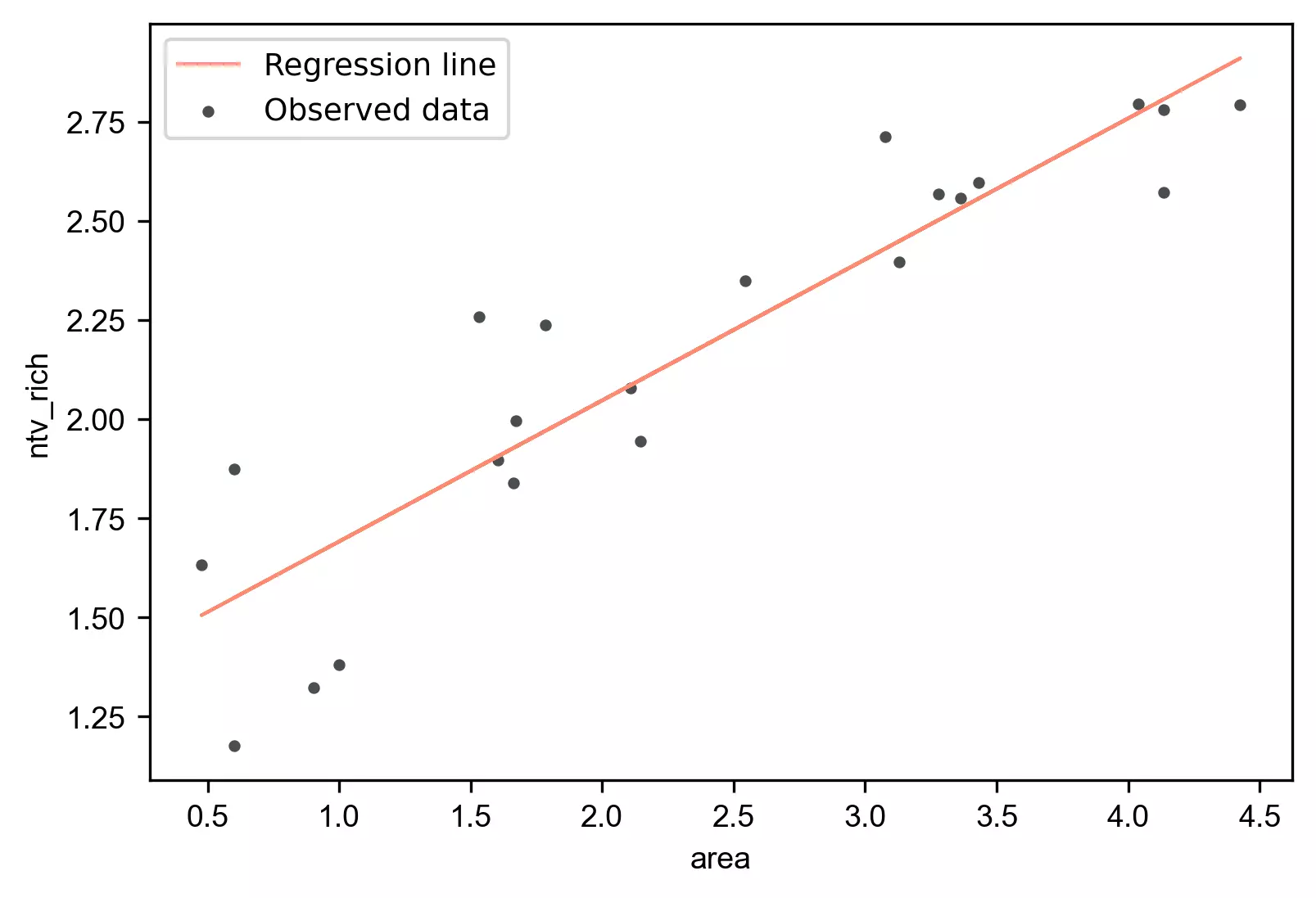
- The regression line with
equation [
y = 1.3360 + (0.3557*area)], is helpful to predict the value of the native plant richness (ntv_rich) from the given value of the island area (area). - Regression can be useful in predicting the native plant richness of any value within the range of the island area. It also predicts native plant richness from area outside the given range, but such extrapolation may not be useful.
Regression coefficients (slope) and constant (y-intercept)
- The regression coefficients or slope (0.3557) represent the change in the
yper unit change in theXvariable. It means the value of native plant richness increases by 0.3557 with each unit increase in island area. - The y-intercept (1.3360)
represents the value of
ywhen theXvariable has a value of 0. Here need to be cautious to interpret the y-intercept as sometimes the value (X=0) does not make any sense (e.g. island area, speed of the car, or height of the person). In such cases, the values within the range ofXshould be considered interpreting the y-intercept. - The p values associated with the
areais significant (p < 0.05). It suggests that the island area significantly influences the native plant richness.
ANOVA
- In regression, the ANOVA tests the null hypothesis that there is no relationship between the independent variable (
X) and dependent (y) variable i.e it tests the null hypothesis that regression coefficient equal to zero (b=0). - From ANOVA F test, the p value is significant (<0.05),
which suggests that there is a significant relationship between native plant richness and island area. The independent
variable (
X) can reliably predict the dependent (y) variable.
Coefficient of determination (R-Squared and adjusted R-Squared)
- The coefficient of determination (R-Squared) is 0.828 (82.8%), which suggests that 82.8% of the variance in
ntv_richcan be explained byareaalone. Adjusted R-Squared is useful where there are multipleXvariables in the model (how to interpret adjusted R-Squared)
Linear Regression (LR) plot
Generate regression plot,
from bioinfokit import visuz
# get predicted Y and add to original dataframe
df['yhat']=reg.predict(X)
df.head(2)
   ntv_rich      area      yhat
0  1.897627  1.602060  1.905964
1  1.633468  0.477121  1.505779

# create regression plot with defaults
visuz.stat.regplot(df=df, x='area', y='ntv_rich', yhat='yhat')
# plot will be saved in same dir (reg_plot.png)
# set parameter show=True, if you want view the image instead of saving
Check Linear Regression (LR) Assumptions
Residuals vs fitted (y_hat) plot: This plot used to check for linearity, variances and outliers in the regression data
# get residuals and standardized residuals and add to original dataframe
df['res']=pd.DataFrame(reg.resid)
df['std_res']=reg.get_influence().resid_studentized_internal
df.head(2)
   ntv_rich      area      yhat   std_res       res
0  1.897627  1.602060  1.905964 -0.040767 -0.008337
1  1.633468  0.477121  1.505779  0.655482  0.127689

# create fitted (y_hat) vs residuals plot
visuz.stat.reg_resid_plot(df=df, yhat='yhat', resid='res', stdresid='std_res')
# plot will be saved in same dir (resid_plot.png and std_resid_plot.png)
# set parameter show=True, if you want view the image instead of saving
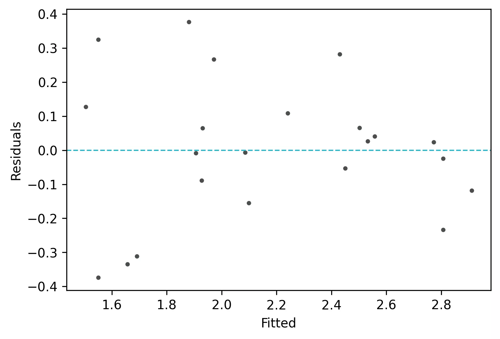
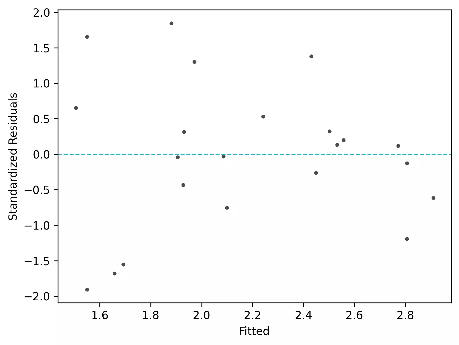
From the plot,
- As the data is pretty equally distributed around the line=0 in the residual plot, it meets the assumption of residual equal variances (homoscedasticity) and linearity. The outliers could be detected here if the data lies far away from the line=0.
- In the standardized residual plot, the residuals are within -2 and +2 range and suggest that it meets assumptions of linearity
Quantile-quantile (QQ) plot: This plot used to check the data normality assumption
import statsmodels.api as sm
import matplotlib.pyplot as plt
# create QQ plot
# line=45 option to plot the data around 45 degree line
sm.qqplot(df['std_res'], line='45')
plt.xlabel("Theoretical Quantiles")
plt.ylabel("Standardized Residuals")
plt.show()
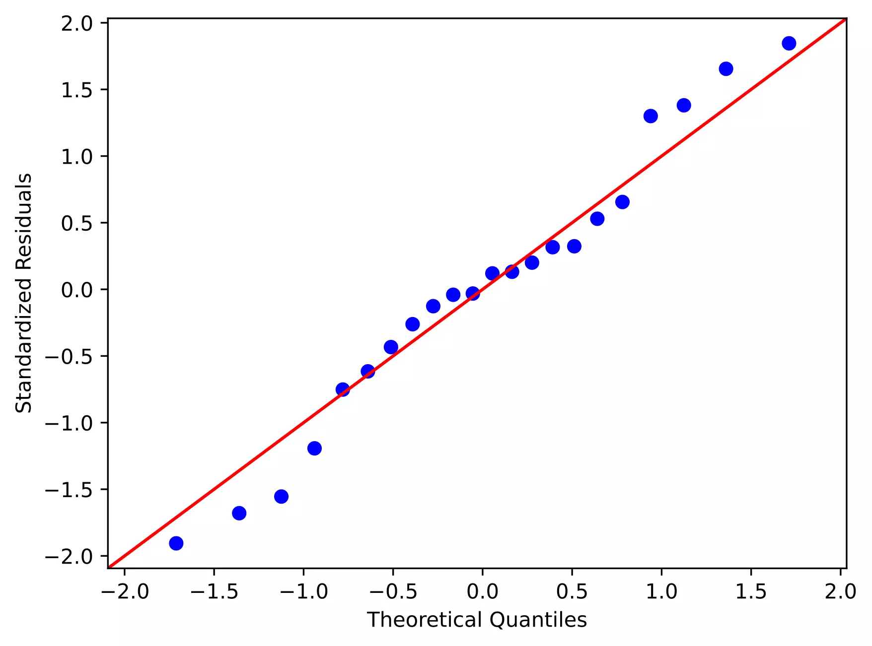
From the plot,
- As the standardized residuals lie around the 45-degree line, it suggests that the residuals are normally distributed
Learn how to train linear regression model using neural networks (PyTorch)
References
- Abdi H. Multiple correlation coefficient. Encyclopedia of measurement and statistics. 2007;648:651.
Related reading
- Multiple linear regression (MLR)
- Mixed ANOVA using Python and R (with examples)
- Repeated Measures ANOVA using Python and R (with examples)
- ANCOVA using R (with examples and code)
- Multiple hypothesis testing problem in Bioinformatics
This work is licensed under a Creative Commons Attribution 4.0 International License